Hydro module
The hydropower system is constructed by connecting hydropower modules into cascades. In the following we describe the module building block in terms of constraints, decision variables and parameters.
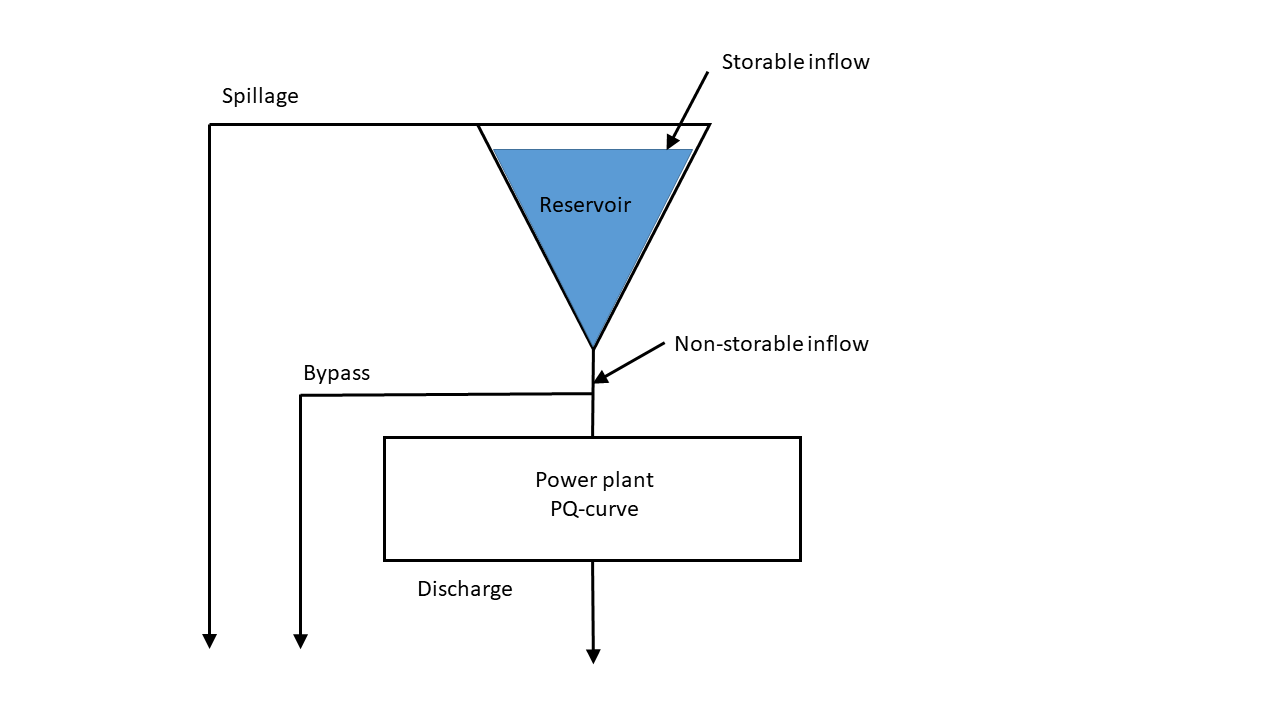
The figure below illustrates a module, comprising a reservoir with a downstream power plant, and with the basic variables involved. Inflow enters the reservoir, while Unregulated Inflow goes directly to the plant. There are three main waterways modeled: discharge, bypass, and spillage. These may be connected to downstream reservoirs or go directly to the sea, and the three waterways are allowed to follow different paths.
Reservoir
Basic Modeling
The reservoir volume for a given reservoir \( i \) in time step \( k \) is represented by a reservoir variable, measured in \( Mm^3 \):
The reservoir volume is bound by the physical limits of the reservoir.
Reservoir Curve
The reservoir curve defines a relationship between the reservoir volume and the corresponding height (m.a.s.l) of the water surface. It is presented as a set of (volume, height) pairs which defines a piecewise linear relationship. The reservoir curve is needed when modeling head dependency in the production function, modeling pumps, and in formulating certain types of environmental constraints.
Reservoir Boundaries
In addition to the physical maximum boundary of the reservoir \( PhysMax(i) \), the user may further bound the reservoir variable by \( ResMin(i,k) \) and \( ResMax(i,k) \). These boundaries are formulated as constraints, and are characterized as soft in the sense that they involve penalty variables.
Minimum Reservoir Boundary
A penalty variable \( res\_viol\_min \) is introduced, measured in \( Mm^3 \):
The minimum volume is set by the constraint MINVOL:
With the following addition to the objective:
where the cost of violating the boundary is given by
which is the input value given by the timeseries minimum_volume_penalty_ts scaled with the reservoir’s energy equivalent and the time step length in hours.
Maximum Reservoir Boundary
A penalty variable \( res\_viol\_max \) is introduced, measured in (Mm^3):
The maximum volume is set by the constraint MAXVOL:
With the following addition to the objective:
where the cost of violating the boundary is given by
\( C_{resViolMax}(i,k) = maximum\_volume\_penalty(i,k) * energy\_equivalent(i,k) * time\_step \)
which is the input value given by the timeseries maximum_volume_penalty_ts scaled with the reservoir’s energy equivalent and the time step length in hours.
Discharge
The discharge waterway represents water going through the power station for the purpose of power generation. After going through the power station, discharged water may follow the path towards a downstream module or go to the sea.
The discharge rate in a module \( i \) in time step \( k \) is represented by a discharge variable \( dis \), measured in \( \frac{m^3}{s} \):
As will be described in relation to the production function for the hydropower plant, the discharge variable is divided into discharge segment variables \( dis\_seg \), measured in \( \frac{m^3}{s} \):
The upper boundaries \( \textrm{MaxDisSeg} \) are found when processing data for the production function.
The relationship between variables \( dis \) and \( dis\_seg \) is ensured by constraint DISVAR:
Bypass
The bypass waterway represents water going outside the power station. Bypassed water may follow the path towards a downstream module or go to the sea.
The bypass rate in a module \( i \) in time step \( k \) is represented by a bypass variable, measured in \( \frac{m^3}{s} \):
If the hydro module has unregulated inflow, the bypass boundaries are increased to ensure feasibility.
To ensure that the bypass variable is not used before the discharge variable (if directed to the same downstream module), we associate a small cost to the use of the bypass variable. By default this cost is less than the cost of using the spillage variable, ensuring that the bypass variable will be used before spillage.
The additional cost component:
Minimum Bypass
Minimum bypass constraints are sometimes needed for environmental reasons. For this purpose a penalty variable \( byp\_viol\_min(i,k) \) is introduced, measured in \( \frac{m^3}{s} \):
With boundaries:
The minimum bypass constraint becomes:
The cost additional cost component:
Note that \( C_{bypViolMin}(i,k) \) must be greater than \( C_{byp}(i,k) \).
Spillage
The spillage waterway should in principle only be used when both discharge and bypass from the module have reached their boundaries. Spilled water may follow the path towards a downstream module or go to the sea.
The spillage rate in a module \( i \) in time step \( k \) is represented by a spillage variable \( spi \), measured in \( \frac{m^3}{s} \):
To ensure that the spillage variable is not used before the discharge and bypass variables (if directed to the same downstream module), we associate a small cost to the use of the spillage variable. By default this cost is higher than the cost of using the bypass variable, ensuring that the spillage variable will be used after bypass.
The cost additional cost component:
Release
If a hydro module has unregulated inflow, i.e., inflow going directly to the power plant, an additional balance is needed downstream the reservoir. To ease the formulation, a new variable \( rel(i,k) \) denoting the total release from the reservoir is defined
The release variable is substituted into the reservoir balance. Reservoir balance without unregulated inflow:
Reservoir balance with unregulated inflow:
Reservoir Balance
The reservoir balance provides explicit control of the reservoir volume. The change in reservoir volume from one time step to the next must equal the difference between inflow and outflow to the reservoir.
To simplify the formulation of the reservoir balance we introduce the collective terms \( FlowFrom(i,k) \) and \( FlowTo(i,k) \). In its basic form \( FlowFrom(i,k) = dis(i,k)+byp(i,k)+spi(i,k) \), while \( FlowTo(i,k) \) is the sum of all water flows from upstream reservoirs directed to reservoir \( i \).
In the special case of k=1, \( res(i,k) = InitialReservoir(i) \)
Tunnels and pumps as special cases.
Hydropower Plant
Terminology and Assumptions
Water discharge is drawn through the hydropower plant to produce electricity. The plant description used in Trident follows the basic principles used in SINTEFs long-term scheduling models:
Plant: Each hydropower module has the possibility of including one power plant. A power plant represents a collection of generating units. The units themselves are not modeled.
Production function: The production function describes the plant’s power output as a function of the discharge. We assume that a production function represent the power output as a piecewise-linear and concave function of discharge. Head-dependency can be modeled, as described later.
The production function is provided as a set of pairs stating power output (\( MW \)) at a given discharge (\( m^3/s \)). We refer to these points as PQ-point and the function is as the plant’s PQ-curve. The \( \textrm{Efficiency} \) per PQ-segment is found based on the PQ-points. If there are \( N+1 \) PQ-points describing the PQ-curve, \( N \) corresponding segments can be found.
If the \( \textrm{Efficiency} \) is strictly non-increasing with segments we have a concave PQ-curve. If PQ-points provided by the user do not meet the concavity condition, these points are removed to ensure concavity.
Production Function
A production variable \( prod\_hyd \), measured in \( MW \):
The relationship between power output and discharge is defined in constraint PRODSUM:
Hydropower production is added to the power balance:
Example: PQ-curve
We assume a plant with three PQ-points: (0,0), (60,20), and (80,40). We need to find discharge segments and efficiencies for two segments.
The discharge variables will have boundaries:
The \( \textrm{Efficiency} \) of two segments:
Tunnel
A tunnel is treated as an additional waterway between reservoirs. The tunnel waterway has a maximum transfer \( \textrm{TunMax} \) that is symmetric in both directions. Since hydraulic pressure is not controlled in the model, the model cannot control whether tunnel flows are according to the law of gravity.
Two variables, \( tun\_from \) and \( tun\_to \), measured in \( \frac{m^3}{s} \):
Where \( F \) is a constant converting from \( \frac{m^3}{s} \) to \( {Mm^3} \)
NB! do we control tunnel capacities wrp initial reservoir levels?
Pump
A pump allows moving water from one reservoir to another, usually upstream.
The pump variable is limited by its maximum pumping capacity \( \textrm{PumMax} \), measured in \( \frac{m^3}{s} \).
Operating the pump requires energy that should be accounted for in the power balance. A constant efficiency \( \textrm{EffPump}(i) \) is assumed.
Using the pumps takes power. So each pump is inserted into the power balance for the corresponding area with a factor that translates pumped water to power usage.
Prior to solving the decision problem, each pump can be deactivated if the difference in reservoir levels for the receiving and sending reservoir is smaller than a defined tolerance.
Scaling pump capacity
Pump capacity \( \textrm{PumMax} \) is scaled according to lift height between the water level of the lower and upper reservoirs. This relation is described as a linear equation \( aX + b \), where x is the lift height. As the lift height increases, a valid scaling of the pump would decrease the total amount of flow through the pump for the same amount of power used.
If relative head scaling is turned off, the above reservoirs nominal elevation is used as the lift height for scaling purposes.
In the power balance the pumps will have the following coefficient:
Note: This calculation only happens at the start of every decision problem. The larger the time span, the larger the difference from the actual behavior of the pump.
Start-up Costs
Variables
\( p(i, k) \) - production of a power plant [in MW]
\( u_{run}(i, k) \in [0, 1] \) - running state of a power plant (can also be defined as binary variable)
\( u_{start}(i, k) \in [0, 1] \) - starting up of a power plant
Parameters
\( P_{cap}(i, k) \) - installed/available capacity for a power plant [in MW]
\( P_{min}(i) \) - minimum production capacity for a power plant [in percentage]
\( C_{start}(i, k) \) - start up costs for each power plant [in unit per MW]
Sets
\( \mathbb{I} \) set of all power plants including hydro and thermal
\( \mathbb{K} \) set of all time steps and scenarios
Indices
\( i \in \mathbb{I} \) - power plant
\( k \in \mathbb{K} \) - time step
Constraints
The running state of a power plant is defined as a variable between 0 and 1. The production of a power plant can between maximum and minimum production, depending on the running state of the power plant, see \( (1) \).
The starting of a power plant is defined by the change of the running state of the power plant, see \( (2) \).
Where InitialState is the state either from input data or from the last time step of the previous decision problem.
Objective function
Start up cost that occur are accounted for, thus they will be included in the objective function.
Volume dependent maximum discharge
Some hydro power plants have a significant connection between discharge capacity and reservoir volume. For these hydro power plants a set of constraints are created that limits the total sum of discharge segments based on input data in the form of a number of RHS, GRAD value pairs that describe a set of linear lines.
As a starting point, we assume that:
The outlet is not submerged (or that the tailwater level is constant).
Head can be expressed as a concave function of volume.
Under these assumptions maximum discharge capacity can be expressed as a concave function of reservoir volume.
For each hydro power plant with a reference to a reservoir for volume dependency, the following constraints are set up:
The values for RHS and GRAD are \( m^3/s \) and \( m^3/s/Mm^3 \) respectively. Meaning that based on a reservoirs volume, a maximum discharge can be calculated. By having the set of lines intersecting to a concave function, the total sum of discharge can be limited for the whole range of reservoir volumes.
Example:
Maximum discharge is 10 \( m^3/s \), represented by the horizontal line at 10. Reservoir volume is between 0 and 100 \( Mm^3 \)
Three points represent the sammenheng between volume and maximum discharge. The three points are:
{0, 0.5}, {5, 0.1}, {9, 0.01}
And the area beneath the lines is the available values for the sum of the discharge segments.
