Flow based market coupling

The introduction of renewable energy sources with low production costs poses challenges related to the efficient utilization of the transmission grid. The standard method of incorporating the physical properties of the grid, the NTC/ATC method, has limited capability in accounting for the actual current flows in market clearing algorithms. As a remedy, the flow based market coupling (FBMC) method has been implemented in the nordic power system.

This section details the mathematical description of FBMC as well as the algorithm and API used in Trident.

Mathematical description

We introduce new variables, \(f_{l,k}\), describing the power flow on line \(l\) at time step \(k\):

\[f_{\ell,k}=\sum_{a}p^{inj}_{a,k} * \Phi_k(\ell,a), \qquad (1) \]

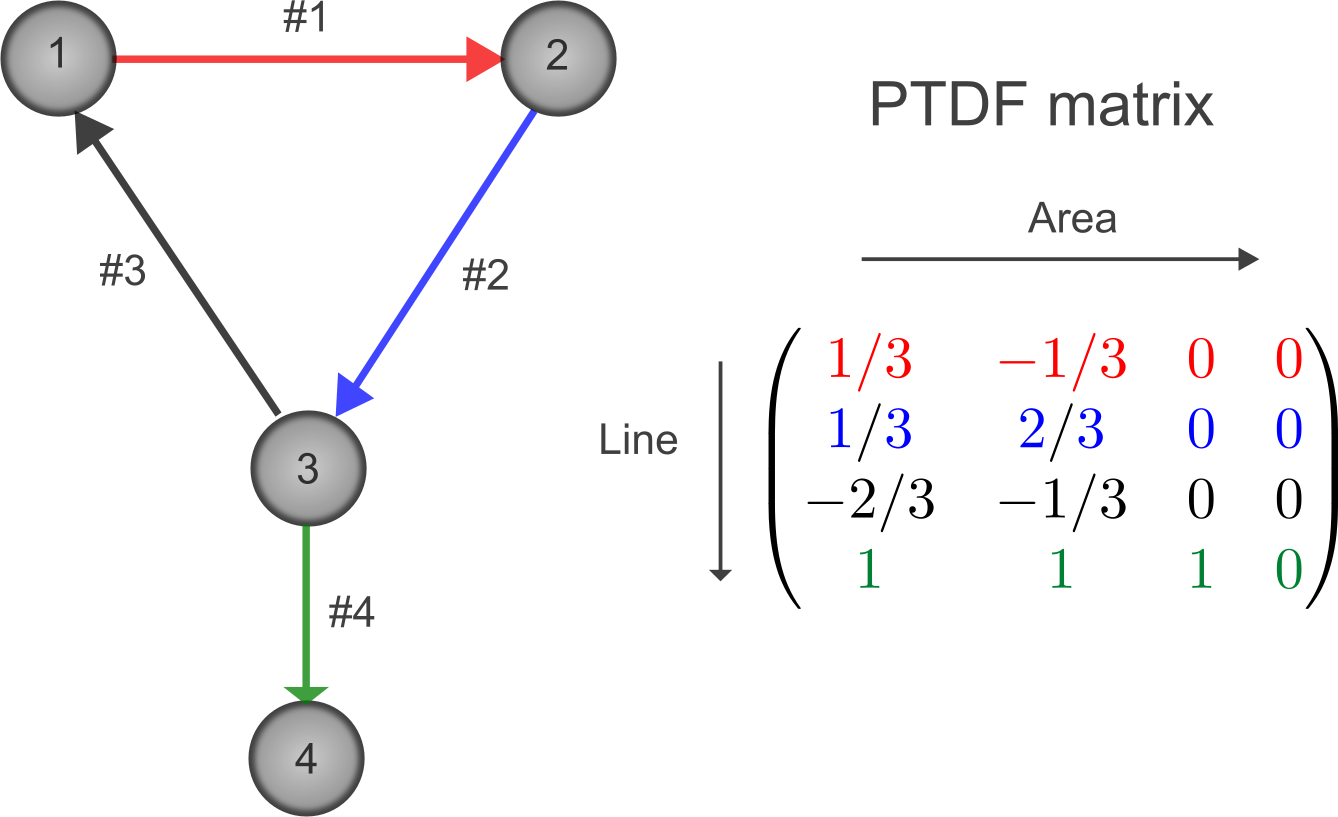
where a is an area index, \(\Phi_k (l,a)\) it the PTDF-matrix with values between \(-1,1\) relating the net injection of area a;

\[p^{inj}_{a,k}=\sum_{\ell \in \mathrm{ACLinesToFrom\;a}} \Bigr( \mathrm{tran\_to}(\ell,k) - \mathrm{tran\_from}(\ell,k) \Bigr) \qquad (2) \]

with the flow on line \(l\). The transmission variables obey the usual constraints:

\[0 \leq \mathrm{tran\_to}(l,k) \leq \textrm{TranMax}(l,k) \qquad (3) \]

\[0 \leq \mathrm{tran\_from}(l,k) \leq \textrm{TranMax}(l,k) \qquad (4) \]

as detailed in the chapter on transmission variables.

New (non-negative) variables, \(f^{viol\pm}_{\ell,k}\), and constraints are added iteratively to the problem in order to satisfy

\[f_{\ell,k} - f^{viol+}_{\ell,k}\leq \textrm{FMaxPos}_{\ell,k} \quad :\mu_{\ell,k}^+ \qquad (5) \]

\[f_{\ell,k} + f^{viol-}_{\ell,k}\geq \textrm{FMaxNeg}_{\ell,k} \quad :\mu_{\ell,k}^- \qquad (6) \]

where \(\textrm{FMaxPos}_{\ell,k}\) and \(\textrm{FMaxNeg}_{\ell,k}\) are the positive and negative line capacities, respectively. \(\mu_{\ell,k}^{\pm}\) are the corresponding dual values of each constraint.

The objective function is modified as follows

\[ \mathrm{Cost}: += \sum_{\ell,k} C_{\ell,k}^+* f^{viol+}_{\ell,k} + \sum_{\ell, k} C_{\ell,k}^-* f^{viol-}_{\ell,k}. \qquad (6) \]

where \( C_{\ell,k}^{\pm}\) are the costs associated with the penalty variables, \(f^{viol\pm}_{\ell,k}\).

Algorithm

Each master problem/week is solved in an iterative fashion: First, we check whether \(f_{\ell,k} > \textrm{FMaxPos}_{\ell,k}\) or \(f_{\ell,k}< \textrm{FMaxNeg}_{\ell,k}\). In this case, we add (3-6) to the LP-problem and solve the master problem again. This process is repated until no new variables or constraints are added. The constraints in Eqs.(3-4) are removed the as soon as the first iteration is done and most of the variables/constraints (5-7) have been added.

System

We here outline the our conventions regarding FBMC applied to a system comprised of four areas with the fourth area/node acting as a “slack node” – i.e., a node which does not provide any injection of current into the system. Adopting a convention of letting rows denote AC lines while the columns denote areas/nodes we have the following intuitive picture: Considering the first column of the matrix, we see that a net position/net injection of 1 MW on node 1 distributes along lines 1,2,3,4 with 1/3, 1/3, -2/3 and 1 MW, respectively.